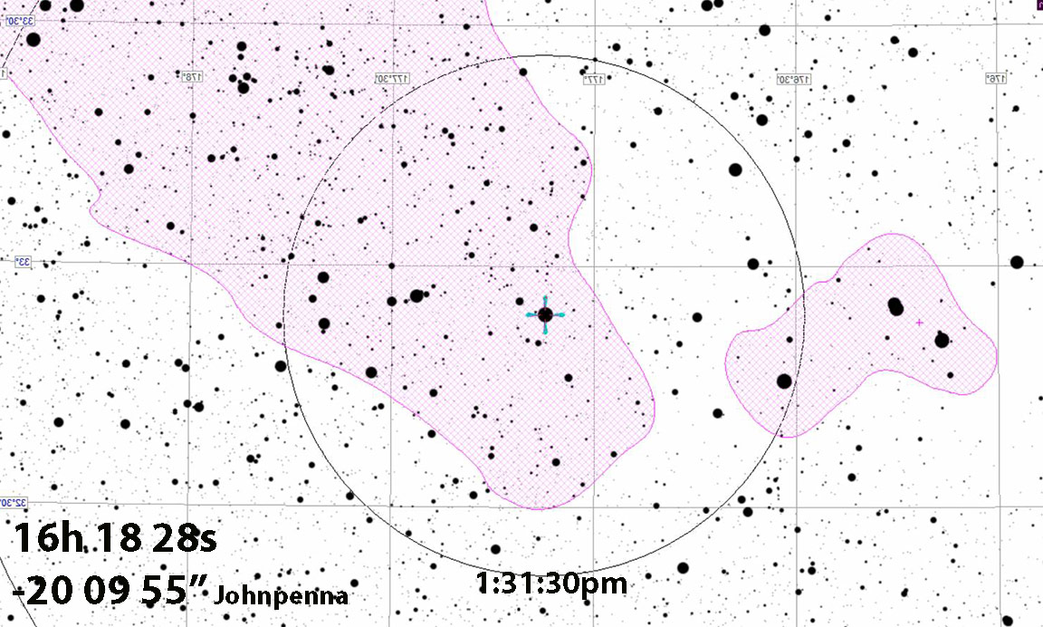
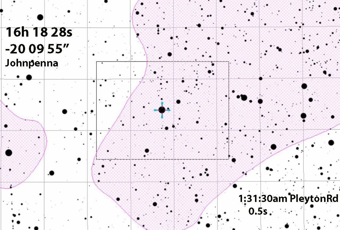
This is a very bright occultation in Scorpius, with a duration of 0.5 seconds and decent altitude for good 1x timing. The target star is very red. IR J-band magnitude 4.0. The path hits too far south along Hwy 1 in Big Sur to make it the favored location, given the road there. Instead, the location best is along Jolon Rd north of Lake San Antonio.
To get the best data, we will want to use 1x and also to reduce gain until the star isn't saturated. By reducing gain, you preserve S/N accuracy while just lowering the counts. This is FAR better than changing gamma, or cutting exposure, or making it far out of focus. Because by cutting exposure, you're hurting S/N with fewer actual photons arriving at their Poisson distributed arrival times. You want instead to count every photon, but scale down the number associated with the count rate. With 1x you can get highest time resolution, and also allow good S/N by cutting gain only.
I've requested a van for Thur May
The weather image looks promising, from ECMWF and Weather.us
click here to see the live cloud image for California
Alt=33, Az=182 due south, just 1 degree left of the top stars in the head of Scorpius.
|
|
A good success. Kirk, Bernard, and I all got usable records of this bright asteroid at high cadence.
Packing up gear at Bernard's Aptos place |
 |
As Kirk is my co-pilot... last minute changes to the sites for maximize efficiency for our three events. |
Sandy's in fine spirits, looking forward to some good science. |
Traffic wasn't fun, though. |
Bernard, prepping his laptop for using his digital Touptec camera and recording. |
Checking my OccBox gear |
Deployment time... |
Arrived; on Jolon Rd south of King City, and Sandy's site, at the turnoff to Ft. Hunder Liggett. |
Kirk checking site maps and path tracks. |
 |
At the site for the Johnpenna event - Sandy is re-deployed - with a funky tripod leg issue. Firm re-insertion and care, it was still functional. |
At Kirk's 2nd site. Quick deploy and then I take Bernard to his 2nd site spot... |
Bernard's digital camera mounted on his 10" f/4 Newtonian. Overkill for a 5th magnitude target star. |
As his camera is not analog, it can't use the IOTA VTI time stamp gear, and so he assembled on a breadboard this 1PPS GPS flash unit |
 |
All seemed to be well, and I drove then to my own site further south. |
Beautiful clean dark dark skies as I awaited Johnpenna. I took some summer Milky Way shots. |
 |
 |
 |
This rather bland shot was to capture those two large trees on the upslope, whom I could ID on the Google Earth images to refine my long/lat. The story of my event is below ... |
Now back to recover Bernard and his expansive gear. |
 |
 |
 |
 |
 |
Kirk, as usual, efficiently got good data on all 3 occultations. Here we're picking up Sandy. Alas, gear trouble again. No data. |
 |
 |
 |
Then the long drive back to Santa Cruz, arriving at dawn. The moon and Venus lit by dawn light |
 |
I set up furthest south, on Interlake Rd. I took photos to document my exact position relative to trees on the GoogleEarth view, after recording my long/lat approximate from my iPhone compass app. GE long lat elev is below:
Long=121 03 57.80s
N. Lat=35 53 44.78"
elev 256m
Too many recent occultations, and it turned out my OccBox battery was too drained to power my gear, but before the event, just as a precaution, Bernard let me borow his spare battery. It was operating on only 26% charge, and this may have meant lower voltage but therefore higher DC current output. Whatever the cause, I had much horizontal Watec row instability in both the VTI numerals and the star image. This prevented OCR of the UT time stamps in PyOTE , which then had to be manually time stamped. Also, processing in PyMovie and PyOTE was very slow perhaps because positioning using time was not possible. I ended up cutting out of the recording just the seconds before, during, and after the event and using just that for my analysis video. I first verified there were no other drops in the PyMovie record which might be due to a moonlet.
The star took about 5 fields to fully disappear, and another ~5 fields to fully reappear, so that a Square Wave timing analysis, as confirmed by Bob Anderson, would NOT provide the correct timings. It must be done in PyOTE with the "edge on disk" (EOD) model. I first had to work through the exact right steps and right values to put into PyOTE in order to help my team then do it with their data.
So reducing the data was problematic. The VTI numerals were too distorted and scrambled to be OCR'd. However, there were enough frames that I could read many of them and be sure of the times, that doing manual time stamps for PyOTE was do-able. Timestamps must be manually inserted each time you run PyOTE. Since I had to run PyOTE many times before I got a solution that was correct. So, here's the manual time stamp data to use: These both include the occultation and check out in PyOTE.
For using the full video, you can use the manual time stamps below...
| Frame | UThr | min | sec |
| 250 | 08 | 29 | 19.0562 |
| 4025 | 08 | 31 | 50.0551 |
But, the very large number of records and time stamp errors makes using the whole video glacially slow in PyMovie/PyOTE. Instead, I've got a trimmed version that just includes a few seconds on either side of the occultation.
For trimmed version, here's the time stamps to use
| Frame | UThr | min | sec |
| 3486 | 08 | 31 | 28.4952 |
| 3543 | 08 | 31 | 30.7752 |
First, here's the Square Wave solution. The PyMovie process is common for both square wave and Edge-on-disk modelling in PyOTE.
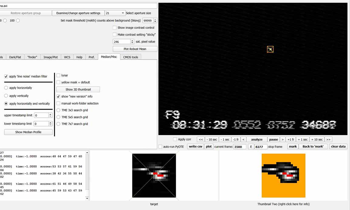
The star was deeply distorted by the poor power supplied to the gear. Not suitable for a circular aperture/mask, as we'll see. |
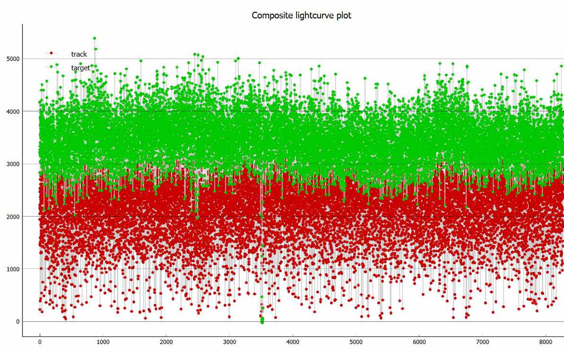 |
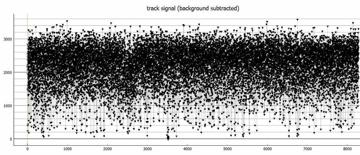
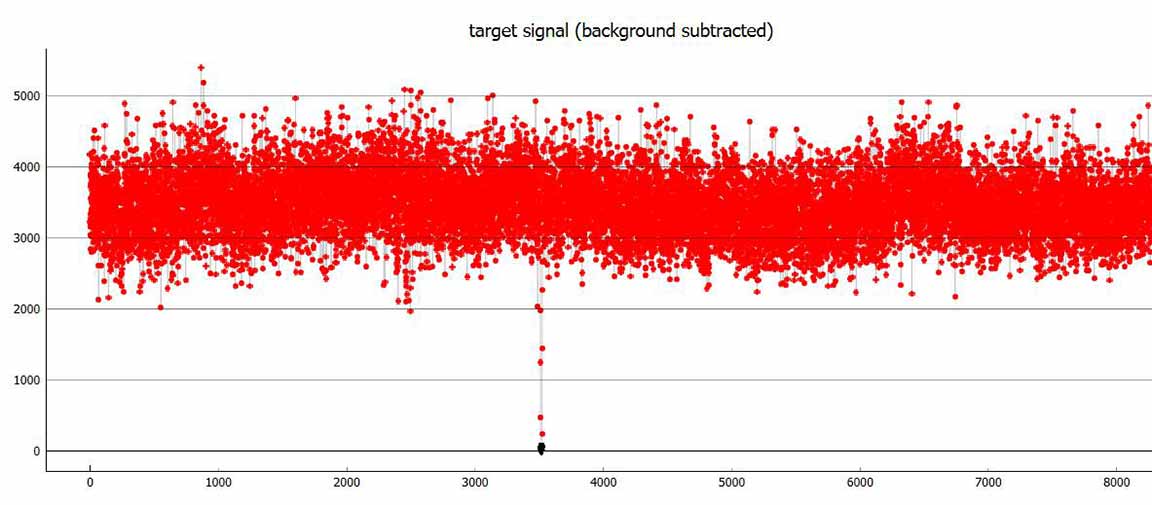
Notice how noisy the signal from the target star is when I use a circular static aperture. |
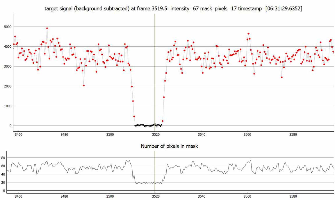
Using a dynamic mask on the same star, is much cleaner. |
 |
 |
|
The solution using the square wave model. Note how the "D" is set at the bottom of the gradual disappearance. |
Still, a genuine occultation is inmistakable. |
magDrop report: percentDrop: 99.6 magDrop: 6.139 +/- 0.861 (0.95 ci)
DNR: 6.75
D time: [08:31:29.4779]
D: 0.6800 containment intervals: {+/- 0.0015} seconds
D: 0.9500 containment intervals: {+/- 0.0037} seconds
D: 0.9973 containment intervals: {+/- 0.0070} seconds
R time: [08:31:29.9939]
R: 0.6800 containment intervals: {+/- 0.0015} seconds
R: 0.9500 containment intervals: {+/- 0.0037} seconds
R: 0.9973 containment intervals: {+/- 0.0070} seconds
Duration (R - D): 0.5160 seconds
Duration: 0.6800 containment intervals: {+/- 0.0022} seconds
Duration: 0.9500 containment intervals: {+/- 0.0049} seconds
Duration: 0.9973 containment intervals: {+/- 0.0085} seconds
Note the duration for the square wave model is only 0.516 seconds. Compare to the edge-on-disk solution which found 0.5601, or 8.5% longer
Edge-On-Disk PyOTE Reduction
I followed the procedure I settled on here: PyOTE Edge-On-Disk Procedure. Here's the parameters from the OWc page and my estimates.
Asteroid diameter: 5.08 mas- 5.7 km
Asteroid speed: 10.67 mas / s
Distance 1.5456 AU
chord estimate: 0.55s
angle=90 since asteriod duration predicted = 0.50 s
Note that the predicted event duration was 0.50s, but the actual duration was 0.55s (square wave) and 0.5601s (EOD). PyOTE would not solve given it required a chord bigger than the asteroid. So, I increased the asteroid diameter far enough that it would not complain. The star diameter is something I had to play with too. If the red curve looked too gentle, I lessened the star diameter. If the red curve couldn't span the points, I increased the chord diameter. If the chord diameter conflicted with the asteroid diameter, I increased both, but only the minimum necessary to avoid complaint by PyOTE. So, the parameters from the OWc predictions above were not the ones settled on to get a good solution. The asteroid diameter had to be increased to 7.1 km or 25% bigger. I also had to increase the initial guess of the star diameter based on the # of points in the D slope and R slope, so from 0.80 km to 1.23 km. The star was therefore 17.3% of the asteroid diameter; enough to justify a disk-on-disk analysis, but the edge on disk is still a very good approximation, given the fact the asteroid was probably not round. I gave it 89 deg impact angles for D and R, and it eventually settled on 90 deg - a central occultation, for both D and R.
Trying to use the entire light curve was glacially slow in PyOTE since almost every frame was unable to be OCR'd because the battery I borrowed from Bernard had critically low voltage and it made for horizontal line noise that was quite bad. It's also why I needed to use a dynamic mask to get the photometric data. So, I trimmed out just the area around the occultation and made that a separate .csv file, which is what I analyzed for the EOD method. Note how now the D and R times are mid way up the falling and rising trend lines; the star center on asteroid edge moments. For square wave, any visibility of the star is considered unocculted, and so the D is then placed at almost the bottom of the drop. This erroneously shortens the duration of the occultation.
 |
 |
For the IOTA report, I use the confidence limits from the SW analysis but insert the D and R times from the EOD method.
Edge-onDisk Final Timings:
D: [08:31:29.4528]
R: [08:31:30.0129]
Kirk and others, please use my new instructions on how to do the "Edge on Disk" method for getting D and R timings. "Edge on Disk" Instructions